Sampling – How to best collect and analyse the sample
The four essentials of sampling
Sampling is one of the most important topics when working with industrial spectroscopy. When searching for a representative analysis of your product
- you need to have a proper representative sample to analyse from and
- the sampling needs to be handled the correct way.
You need to get these four aspects right to get a proper representative sampling result:
- Physical sampling – How to get a sample in real life
- Sampling in time
- How to present a sample to a NIR-analyser
- Optical scanning – How to take the spectrum
These are the four aspects of how to take a high-quality representative spectrum and obtain a precise representative analysis of your product.
1. Physical sampling – How to get a sample in real life
The first important aspect of sampling is physical sampling, also called practical sampling. Sampling can be viewed as the steps you need to go through to battle the unavoidable heterogenic (non-uniform) nature of most products and processes.
A given concentration of a constituent in your product is not constant over time.
Meaning that at a given time all particles in your product are not equally represented in the sample. At the same time not all particles of the product are equally accessible.
Revealing the true chemical composition of a sample by FT-NIR is not trivial, even though it may be very easy to reach some kind of result in seconds. It is even less trivial to prove that not only do you know what is in the sample, but this information speaks for an entire field, tank, truckload, or process state.
Understanding the essence of proper sampling requires but one fundamental principle to be followed, known as the Equal Probability Paradigm. Written simply, the principle is that all particles/parts must have the same (non-zero) probability to influence the spectrum on which a later prediction will occur.
The practical world will present us with a few more challenges than can be fixed with this one rule. Let us look at a few of the challenges to get an understanding of what a Quant or InSight Pro system must handle. For a full understanding, we encourage further study of the theory of sampling.
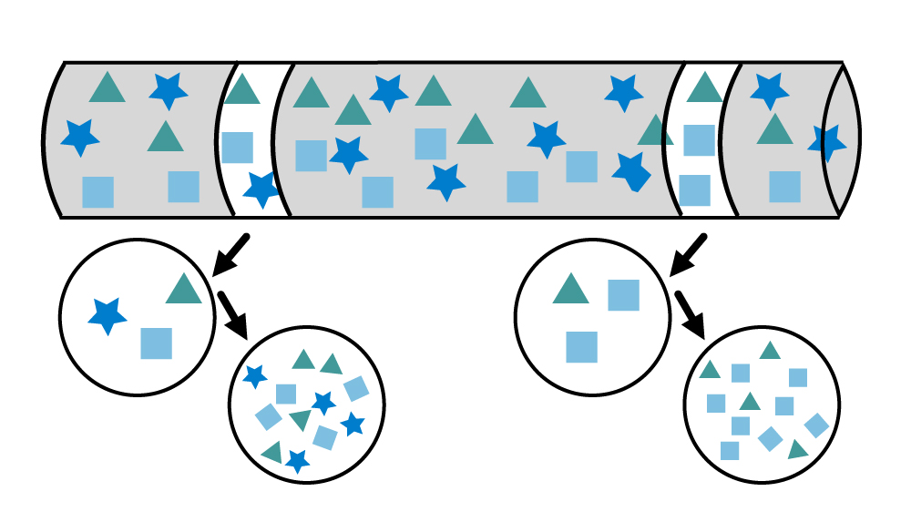
The heterogeneity will often present itself in two basic expressions. In the Theory of sampling (TOS) we denominate these DH and CH, short for Distributed vs Content Heterogeneity.
Distribute Heterogeneity means simply that a given concentration is not constant over time, whereas Content Heterogeneity means that all particles at a given time (t) are not equally distributed in the sample. This is illustrated below, where the two slices represent samples taken at different times, and the cross-sections show content heterogeneity of the particles in these two samples.
All particles/parts must have the same (non-zero) probability to influence the spectrum on which a later prediction will occur.
Another fundamental challenge is what we could call the accessibility challenge for our sampling. To really follow the equal probability paradigm, all particles must be equally accessible and that is fare from true in most cases.
The theory of sampling operates with dimensionality, with four possible dimensionalities. Of these, three are practical (1D, 2D and 3D) and one is the ideal but hypothetical scenario of 0D.
A tank, truck, ship or pile is seen as three-dimensional, whereas a green-field is seen as 2D and we generally think of smaller pipes as one-dimensional.
Needless to state that if you place your self on the edge of a ship and wish to acquire a single sample from the ocean, you are more likely to sample the top surface than any other place and hence what is hidden at the bottom will stay hidden to you, but will eventually reach the process as an unknown factor because it has not been sampled before.
Anyone who ever sat on a harvester knows this and everybody else can quickly build a good intuitive sensation of the fact that the protein or moisture content is not the same all over the field. The low, pitted stretch may show a higher moisture content than the parts growing in the sandy areas of the field. Taking just one simple sample will not tell us what the content may yield in total or per hectare.
Sampling a conveyor belt or powder stream is truly a challenge which must be met with respect and proper science to yield highest quality analytical result.
All the above is necessary to ensures that the FT-NIR spectrum obtained is representative, and only chemometric models based on representative samples/spectra/variation should be used for calibration and measurements.
A major common error is to extract one sample of X grams which fits directly in the analyser. The error can be divided into several sub errors.
Firstly, we should never just “grab a sample” and trust this singularity in time. It would be as wrong as to ask the first voter in a public referendum and make this answer the official result. Here we all know that hundreds if not thousands of voters need a saying before we get an idea of the outcome of the election. Sadly, quite often the process gets “asked” only once.
If we wish to battle especially content heterogeneity at a given time (see below) we need a composite sample – this is also a fundamental rule. Take a few subsamples from “all over” – mix them and from that take one or maybe a few sub-samples and run them through the analyser. The average result will be a much better estimate of the current process state!
It is typically not done, due to time restrictions – but getting to the wrong result fastest will never be a priority for Q-Interline.
In summary, the highest quality analytical results demand that:
- Samples extracted for analysis are representative
- All mass reduction (sub-sampling), handling and preparation must follow strict protocols – which ensure representativity
- Sample presentation to the analyser must be representative
- Optical scanning of the sample must be representative
2. Sampling in time
Sampling in time is relevant for both laboratory units like the Quant and for the InSight Pro in-line systems. The core question is how often one should analyse to know enough to control the process and hence the product quality, overall yield and income. There are multiple answers to this question and many considerations to entertain, but here we will stick to a sampling perspective of the challenge.
In many practical aspects a sample is taken every X minutes or hours, indifferently of the process variation and only rarely based on statistics.
In principle, this theme is about handling distributed heterogeneity and acceptance of the fact that processes are not stable.
Let’s review the below example. The dataset is a simple creation of a process scenario in which 3 sinusoidal curves have been overlaid with an element of noise added. The total time is 120 minutes.
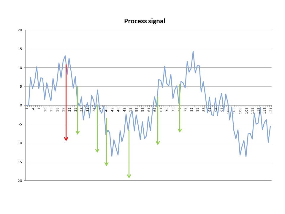
The process is in principle over time stable around 0 offset from target, but a certain dynamic is present, and the effect of the time of sampling becomes evident.
If a sample is drawn after 20 minutes (red arrow) the QC function would conclude that the process is running some 12% off target. If the operators would then tune down the process at that time the process would no longer reach a zero-average error over the 2 hours.
If we sample more often the process dynamics may be revealed (green arrows) and with better insights it is possible to make better decisions. If the process is not stable over time, this argues for an InSight Pro solution over the laboratory units.
3. Presenting the sample to the analyser
It will all be of little or no use to acquire a perfectly representative sample in time, space and all dimensionalities if, at the end, the sample is not presented to the analyser in a proper way.
It may seem that by going on-line we skip a lot of problems, but keep in mind that the on-line analysers see the process through a relatively small probe which can be equivalated to a man studying the world through binoculars – we better point him in the right direction. Likewise, a process analyser must have the probes and cells placed in a proper position to sample the process correctly. Consider the case of powder sampling: one must avoid sampling only the fine particles or only the coarse particles, otherwise it risks an overrepresentation in the measurement.
Our laboratory Quant units can handle nearly all sample types, by proper choice of sampling device (accessory). We offer accessories supporting different physical set-ups from clean transmission to diffuse transmission and diffuse reflection in several variations.
| Physical principle | Sample types | Q-Interline accessory |
|---|---|---|
| Transmission | Clear liquids | Vial Sampler |
| Diffuse transmission | Liquid dairy products | DairyQuant GO |
| Diffuse reflection | Solid/semi-solid and powder dairy products | Cup Sampler / Petri Sampler /Bottle Sampler |
| Diffuse reflection | Soil and compost | Bottle Sampler |
| Diffuse reflection | Silage and hay | Spiral Sampler |
The InSight Pro unit with five different probe and cell configurations can be adapted for a wide range of process streams applying the same physical principles as for the Quant solution for at-line.
| Physical principle | Sample types | Q-Interline accessory |
|---|---|---|
| Transmission | Clear liquids like edible oils, water, chemicals | Probe sampling / Cross pipe cell |
| Diffuse transmission | Liquid dairy products | Cross pipe cell |
| Diffuse reflection | Semi-solid or pasty dairy products | Reflectance Probe |
| Diffuse reflection | Semi fine powders | Spoon Probe |
4. Optical scanning
Optical scanning is the final discipline to master in sampling to acquire optimal spectral data which, if combined with premium quality reference chemical data, will yield great results with minimum effort.
All Q-Interline systems can be thought of like a camera. You may go with the settings we have found most optimal in most cases for the specific application (auto) or you may endeavour into a world of settings and options (manual) – the latter for the specialist only, but it may perform better than auto in some cases.
Very much in line with the “public referendum” idea in the chapter of physical sampling, here in optical sampling we should also apply the fundamental principles. All particles should have the same chance of becoming part of the spectrum and we need to accept CH.
This means that all sampling options from Q-Interline intended for heterogenic samples will argue not to look at a small spot but rather the entire sample. For on-line systems, the sample is moving past the probes and cells and by tuning observation time we create a spectrum of a given “area”. All laboratory models measuring with reflection will typically spin or even tumble the sample and in this way deliver on the promise to obey the fundamental sampling rules.
Once the sample is moving, we still have several parameters to play with.
The first is the resolution. This is a fundamental difference between adjustable resolution with the base Quant engine of Q-Interline and products based on diode array or dispersive technology where resolution is fixed.
Resolution is the ability to separate to adjacent peaks in the spectrum. Be careful, the band shape of peaks in the NIR region are very broad and overlapping and can only very rarely be resolved and overdoing the resolution will only lead to noisy data. All Q-Interline systems can run with resolution from 1-128 cm-1. Most applications of Q-Interline uses a resolution of 32 cm-1 which means a datapoint spacing of 16 cm-1 which is more than enough to get all details at very low noise.
| Resolution | Scans per min. |
|---|---|
| 8 | 37 |
| 16 | 75 |
| 32 | 150 |
| 64 | 250 |
The next parameter is measurement time and the number of scans to co-add into the final spectrum. The number of scans per second varies with resolution, so represents a trade-off: less resolution allows for faster sampling and vice versa. Below a few examples
The number of scans can be freely set for online, but we recommend setting observation time so that repeatability is the minor factor in the total error budget.
For Quant units with a spinning accessory, the number of scans and observation time, are set to match one or two full rotations, but never fractions of rotations! If we run 1.5 turns in a Petri Sampler, half the sample will have contributed twice as much to the measurement, and that would be a gross violation of good sampling practice.
We create value for you
Our vision is to be the best provider of FT-NIR analytical solutions in the world. We help our customers:
- Ensure product quality
- Optimise raw material utilisation
- Optimise production processes
- Reduce energy consumption
in an easy, precise, and efficient way with our patented FT-NIR solutions.
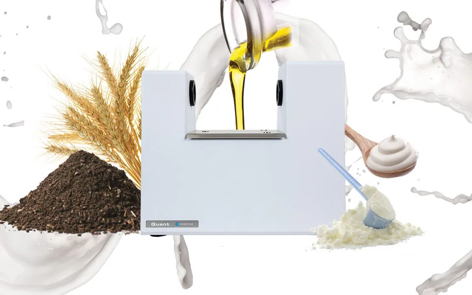
We work with customers within dairy, agriculture, food and ingredients and in the Nordics also within pharma and chemical.